
Introduction
SADDLE is a tool to design cluster supercomputers and data centres. It can design HPC clusters, Hadoop clusters, web server farms and other types of large and small data centre hardware. It will calculate performance, cost and technical metrics for you automatically, providing you with a ready bill of materials you need to buy.
SADDLE stands for “Supercomputer And Data-centre Design LanguagE“. It’s a Python-based language, operated either interactively or with a script. If you need a 10-minute introduction, see this presentation made at the International Supercomputing Conference (ISC’14) in Leipzig, Germany.
SADDLE is modular; you can mix-and-match existing modules or create your own, such as performance models.
Download
SADDLE is packaged as part of Cluster Design Tools, please refer to “Download” on how to download and install the tool set. Run the tools as specified in that document and make sure that they work, then return to these instructions. Change to the directory with SADDLE files (bin/saddle/) and find the main file, “saddle.py”. We will later run SADDLE interactively by calling this file.
Design Workflow
To design a cluster supercomputer, we need to perform several stages:
- Choose the problem to be solved, and choose (or create) a performance model
- Choose compute node configuration (use constraints and heuristics)
- Calculate the required number of compute nodes
- Configure the network and the uninterruptible power supply (UPS) system
- Place equipment into racks, locate racks on the floor
- Calculate cable lengths
- Do the economic part of calculations
- Print design documents
SADDLE tackles these challenges by orchestrating the query of corresponding modules from the Cluster Design Tools and combining their results.
First Steps
Choose Compute Node ConfigurationChoose Compute Node Configuration
Let us reproduce the results from the SADDLE presentation (the link to the PDF is in the beginning of the page). We will execute, step by step, the example script included with SADDLE distribution. The difference is that we will run commands interactively rather than launch a single script. You can simply copy and paste commands below and observe the results.
Let’s start with running SADDLE in interactive mode:
python -i saddle.pyRunning on Linux?
If you are using Linux, then you may have a previous generation of the Python language already installed, called version 2, that will be invoked when you call “python”. Since for SADDLE you need Python ver. 3 (the exact suitable version is specified in “Download”), you need to use the command “python3” instead of just “python”:
python3 -i saddle.py
A welcome banner appears, followed by a standard Python prompt (“>>>”). Here, we can start typing commands. The first command will open the database of available compute nodes:
open_db(['db/generic.xml', 'db/generic-server.xml',
 'db/intel-xeon-2600.xml', 'db/intel-xeon-phi.xml',
 'db/memory.xml', 'db/network.xml', 'db/hdd.xml',
 'db/ssd.xml'])
If the Cluster Design Tools are already running in the background (and they should be), SADDLE will send the database files you specified for processing. The result is the set of available hardware configurations for compute nodes:
> Database opened
> Enabled configurations: 448 of 448
> No undo steps
So, compute nodes can be configured in so many different ways. Let us impose constraints; first, we will require that configurations have InfiniBand network adapters:
constraint("'InfiniBand' in network_tech")
Half of configurations now remain:
> Constraint(s) "'InfiniBand' in network_tech" imposed
> Enabled configurations: 224 of 448
> 1 undo step(s) available
Now, let us also require that compute nodes have exactly two CPUs installed:
constraint("node_cpu_count == 2")
This leaves us with even fewer configurations:
> Constraint(s) "node_cpu_count == 2" imposed
> Enabled configurations: 112 of 448
> 2 undo step(s) available
Now, let us see how many memory per core these configurations have:
> Statistics on metric "node_main_memory_per_core"
 computed over 112 enabled configuration(s):
> Minimal value: 2.7
> Median: 4.25
> Maximal value: 6.4
Suppose the codes we are going to run on this machine don’t need much memory. Let us select only configurations with the lowest amount of memory per core. By default, “select_best” will search for the minimal value of metric, which is just what we need. (Note: if you had specific requirements on memory size, you would instead specify them with a “constraint” statement).
select_best("node_main_memory_per_core")
We still have quite many configurations, because there are things like CPUs, storage and accelerators that we have not yet configured:
> Best configuration according to metric "node_main_memory_per_core"
 selected
> Enabled configurations: 16 of 448
> 3 undo step(s) available
Let us specify that we want compute nodes to have three Intel SSD drives:
constraint("ssd_count == 3")
Now, we have 8 configurations:
> Constraint(s) "ssd_count == 3" imposed
> Enabled configurations: 8 of 448
> 4 undo step(s) available
These example compute nodes can be equipped with zero, one, two, or three Intel Xeon Phi accelerator boards. Let us ask to have no accelerators in this machine:
constraint("accelerator_count==0")
As the result, only two configurations remain (they differ in CPU models used):
> Constraint(s) "accelerator_count==0" imposed
> Enabled configurations: 2 of 448
> 5 undo step(s) available
Now, we could choose the CPU that either has the highest performance or the lowest cost, but that would be simplistic and unreliable. Let us instead refer to the more advanced technique and calculate a custom metric, the cost/performance ratio of the compute node, and then choose the configuration with the lowest value of this metric:
metric("node_cost_to_peak_performance = node_cost / node_peak_performance")
Metric value is calculated for both configurations, and statistics are automatically printed:
> Metric(s) "node_cost_to_peak_performance =
 node_cost / node_peak_performance" calculated
> Statistics on metric "node_cost_to_peak_performance"
 computed over 2 enabled configuration(s):
> Minimal value: 34.50617283950618
> Median: 36.0595100308642
> Maximal value: 37.61284722222222
> Enabled configurations: 2 of 448
> 6 undo step(s) available
It’s time to choose the best of the two configurations, based on this metric:
select_best("node_cost_to_peak_performance")
Finally, only one configuration remains:
> Best configuration according to metric
 "node_cost_to_peak_performance" selected
> Enabled configurations: 1 of 448
> 7 undo step(s) available
We can now delete all inferior configurations and save the result in a CSV file. This way, we can later load this file without having to impose constraints and apply heuristics:
delete()
save_db('generic_server_best.csv')
All done, database saved:
> Disabled configurations were deleted
> Enabled configurations: 1 of 1
> 8 undo step(s) available
> Database saved
Now, take a break and open the resulting CSV file in your favourite text editor or in a spreadsheet. You will see that a configuration of a compute node is determined by its metrics which are stored in key-value pairs. In a spreadsheet, the column title is the name of the metric, and the cell below the name is the value of that metric. That’s how it looks in OpenOffice Calc (click to magnify):
Resulting CSV file when opened with OpenOffice Calc
Not tired yet? Let’s move on to more interesting things!
Determine the Number of Compute Nodes
In this section, we will use an inverse performance model to calculate the number of compute nodes in a cluster required to reach a specified performance level. We assume that your SADDLE interpreter session is still running; if yes, exit it, like you would exit any interactive Python session:
exit()
Now, launch a new SADDLE session (“python -i saddle.py”) and load the CSV file that you saved at the previous step, using this command:
open_db('generic_server_best.csv')
Cluster Design Tools currently implement only one performance model — that of ANSYS Fluent 13, a computational fluid dynamics software suite. The link to query this model is already wired into SADDLE and is stored in the Python dictionary that has the name “inverse_performance_module”, under the key called “url”. You can even print it using this simple Python statement:
print(inverse_performance_module['url'])
This returns the following URL that would be used to query the corresponding performance module:
http://localhost:8000/cgi-bin/performance/fluentperf/fluentperf.exe
 ?task=design&benchmark=truck_111m&allow_throughput_mode=true
If you tried to copy and paste this URL into your web browser, you would see that the performance module is queried but returns an error. That is because SADDLE appends many parameters to the URL before query, thereby passing information into the module.
Running on Linux?If you are trying SADDLE on Linux, you would notice the “.exe” extension in the URL. That’s for Windows users, and we would need to strip that on Linux. The best interim solution would be to open the main file, “saddle.py”, in editor, scroll down until the end, and find declarations of Python dictionaries called “performance_template” and “network_module”.
There, find the key “cUrl” and delete “.exe” from the long strings stored under that key. For example, “…/fluentperf.exe” would turn into just “…/fluentperf”. Save the file and restart SADDLE. It should work now: the above “print” command should print the URL without the “.exe” extension.
If you created your own performance module compatible with SADDLE’s conventions, you can specify its URL by assigning it to the data structure:
inverse_performance_module['url'] = "http://example.com/cgi-bin/my-perf-model"
But if we are happy with the choice of the default performance model, let’s just query it. We specify the performance we want to achieve on this machine, in tasks per day:
inverse_performance(240)
SADDLE immediately connects to the performance module and queries it. It means the module should already be running and awaiting connections, that’s why we launched Cluster Design Tools before running SADDLE. The output looks like this:
> In configuration 391, you now have 336 cores in 14 nodes,
 with 24 cores per node
> Number of cores and nodes calculated
> Enabled configurations: 1 of 1
> 1 undo step(s) available
What happens during the module query is that new key-value pairs are returned by the module and then injected into the configuration we work with. In fact, you can examine configurations using SADDLE function called “display()”, supplying to it the number of the configuration you want to display. Since we loaded a CSV file that contains only one configuration, we specify number one here:
display(1)
This produces a long list of key-value pairs that store the metrics of our future cluster computer. You are encouraged to scroll your screen to examine them. In particular, the performance module calculated the required number of CPU cores and returned it as “cores”, and then SADDLE calculated the number of compute nodes and stored this as “nodes”:
...
cores=336
...
nodes=14
...
(For the curious: there was actually one more step involved: after calculating the number of compute nodes, SADDLE rounded up the number of CPU cores and called the performance module another time, this time supplying it with the number of cores rather than required performance. The performance module returned the updated performance figure: “performance=241.4”. This number is always slightly higher than the performance of 240 tasks per day that we originally requested, thereby making sure that our cluster is at least as fast as we asked it to be).
Adding network and UPS system
Every decent cluster supercomputer needs an interconnection network. Nothing could be easier but to design one with SADDLE. Assuming you are still at the interactive SADDLE prompt, issue the following command:
network()
Here is the output:
> Network designed
> Enabled configurations: 1 of 1
> 2 undo step(s) available
Now, wasn’t that easy? SADDLE queries the network design module, receives corresponding metrics and injects them into the current configuration. You can examine the configuration by using the command “display(1)”, as you did previously, and scrolling your screen. Pay particular attention to metrics that start with “network”. You will notice that a star network has been designed, with a 36-port switch. This is as expected, since we only have 14 compute nodes, and a fat-tree network is not required:
network_blocking_factor=1
network_core_switch_count=0
network_core_switch_model=N/A in star networks
network_cost=11580
network_edge_ports_to_core_level=0
network_edge_ports_to_nodes=36
network_edge_switch_count=1
network_edge_switch_model=Mellanox SX6036 (36 ports)
network_edge_switch_size=1
network_expandable_to=36
network_power=207
network_tech=InfiniBand
network_topology=star
network_weight=8
The uninterruptible power supply system, or UPS, can be designed with a similarly simple statement. The UPS design module will be queried:
ups()
You can actually omit this step if you don’t want a UPS system. But if you issued the above command, the output would look like this:
> UPS subsystem designed
> Enabled configurations: 1 of 1
> 3 undo step(s) available
The metrics have been supplemented with the following:
ups_backup_time=2940
ups_cost=35000
ups_heat=900
ups_model=Liebert APM (up to 45kW)
ups_partitioning=1*15000
ups_power_rating=15000
ups_size_racks=1
ups_weight=417
So, we have here one UPS block that takes up one rack and provides up to 15 kW of power. That’s the minimal power capacity block we have in the UPS database, and our cluster will actually consume only 7,7 kW of those 15 kW, so it’s sort of over-provisioning.
Placing equipment and laying cables
Now as we have added all necessary computing, network and UPS hardware, we can place it into racks and locate racks on the floor. We need to specify the name for the group of equipment to be placed; this name will later appear on drawings:
add_group('compute')
SADDLE will inform you which subgroups of equipment it created:
>> Created 1 group(s) of servers
>> Created 1 group(s) of edge switches
>> Created 1 group(s) of UPS equipment
> Group "compute" added
Each of these subgroups will be denoted by its own colour in drawings. Now it’s time to place all this equipment into racks. The default strategy is to place equipment as densely as possible:
place()
After equipment is placed into racks, racks are located on the floor, and SADDLE queries the floorplanning module to determine clearances around racks. In response, SADDLE prints the number of rack-mount units that the hardware will occupy:
>> Placed all 57 units of equipment successfully
> Equipment placed into racks; design-wide metrics updated
In this case, 42 units are for the UPS system that takes one rack, and the remaining units are 14 for servers and 1 for the network switch. When all subgroups of equipment have been placed into racks, and their locations within racks are also known, we can lay out cables:
cables()
SADDLE replies with a terse message:
> Cables routed
It would be interesting to see what the results looks like! And we are coming to it soon.
Getting design documents
To print the design documents in text format, you can use the following command, optionally specifying the file name as an argument:
print_design('generic_server.txt')
The reply informs you of successful save:
> Design information saved to file "generic_server.txt"
We will take a look at the contents of this file in the next session, and will now proceed to drawing the front view of racks, which is performed with the following statement:
draw_rows('generic_server.svg')
SADDLE will let you know if everything went well:
> Rows drawn
Now it’s time to open the resulting SVG (scalable vector graphics) file with the software of your choice. If you have Mozilla Firefox, you can drag-and-drop the file into its new window; it’s more than enough for viewing the drawing. If you would like to make edits, I would recommend using Inkscape. Our particular cluster only has 14 compute nodes and does not look very spectacular. The green line on the diagram represents all 14 cables that connect compute nodes to the switch:
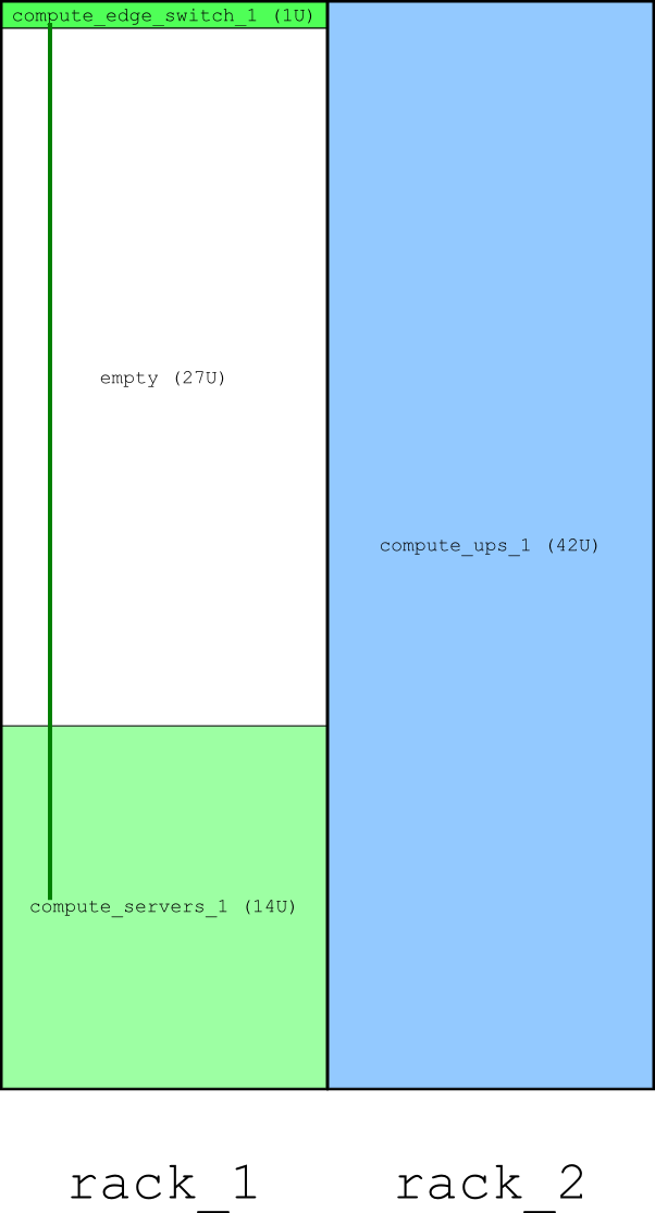
Computer cluster designed by SADDLE, for 14 compute nodes (240 tasks/day with ANSYS Fluent 13 benchmark “truck_111m”)
Understanding Design Documents
Let’s decipher SADDLE’s output that we earlier saved to a text file, “generic_server.txt”. There are several sections in that file: open it in your preferred text editor, and you will see for yourself.
Groups of EquipmentThis section lists groups of equipment which you previously added with the add_group() statement (in the example above, we added only one group, but there is a potential to add more). For each group, we can see the number of compute nodes, peak floating-point performance for one node and for the whole group, and power consumption of the group:
       Groups of Equipment (1 group(s) total)
       --------------------------------------

1. Group "compute"

Number of compute nodes: 14
 Compute node model: Generic server
 Node peak performance: 518.4 GFLOPS
 Group peak performance: 7.26 TFLOPS
 Group power: 7.73 kW
What follows is a meticulous enumeration of all possible characteristics of equipment in the group. Basically, you can send this output to your equipment supplier to indicate what you want to buy:
 Node form factor: Rack-mount
 Node cost: 17,888
 CPU model: Intel Xeon E5-2697 v2
 CPU clock frequency, GHz: 2.7
 Cores per CPU: 12
 CPU count: 2
 Node power: 473 W
 Main memory:
   Size: 64
   Type: PC3
   Speed: 12800
 Network:
   Topology: star
   Cost: 11,580
   Edge switches:
     Model: Mellanox SX6036 (36 ports)
     Count: 1
     Size, RU: 1
 UPS System:
   UPS model: Liebert APM (up to 45kW)
   Backup time: 2,940
   Power rating: 15,000
   Partitioning into blocks: 1*15000
   Size (racks): 1
   Weight: 417
   UPS cost: 35,000
 Economic characteristics:
   Capital expenditures: 297,012 (91.84% of TCO)
   Operating expenditures: 26,405 (8.16% of TCO)
   Total cost of ownership: 323,417
This section lists the results of equipment placement. The number of racks is printed, their size in rack-mount units, physical dimensions and clearances.
The floor size, as well as the “row formula” which determines how many rows you have and how many racks are in a row, is calculated by the floorplanning module:
                   Racks and floor space
                   ---------------------

Rack count: 2
Rack size, in rack-mount units: 42
Rack physical dimensions and clearances:
  Width: 0.6
  Depth: 1.2
  Height: 2.0
  Side clearance: 1.0
  Front and back clearance: 1.0
  Aisle width: 1.0
  Maximal length of row segments: 6.0
  Overhead tray elevation: 0.5
Floor space:
  Dimensions: 3.2 x 3.2
  Size: 10.24
  Rows of racks: 1
  Racks per row: 2
  Row formula: "2"
This one is easy: it lists cables you need to buy, and their total length:
                Bill of Materials for Cables
                ----------------------------

Length    2:      14 cable(s)

Total number of cables to order:      14
Total length of all cables:           28
In this case, you need 14 cables, one per each compute node. All cables are the same (look at the cabling diagram above), the length of each is 2 metres, so the total cable length is 28 metres.
The last section summarises everything; it collects all important macro-level characteristics in one convenient place. First, there are constants which are used to calculate operating expenditures: system lifetime, electricity price and rack stationing costs (the price of renting space for one rack):
                    Design-wide metrics
                    -------------------

System lifetime, years:             3
Electricity price per kWh*hour:     0.13
Rack stationing costs per year:     3,000
Next come capital and operating expenditures, and the total cost of ownership, which is the sum of the two. The share of each type of expenditures — capital and operating — in the TCO is clearly indicated. Sometimes it leads to unexpected revelations that energy costs are not really as big as they are usually perceived:
Capital expenditures:               297,012 (86.99% of TCO)
Operating expenditures:             44,405 (13.01% of TCO)
Total cost of ownership:            341,417
Finally, the total power consumption is given (how many watts you need to request from your data centre facility), as well as the “tomato equivalent” and the weight of your machine, should you decide to move it to another data centre one day (or if you want to calculate floor load).
The “tomato equivalent” deserves a special explanation: it is the amount of tomatoes that you can gather each day if you reuse all waste heat from your computer for heating a greenhouse. Read more here about how it is calculated: “Fruits of Computing: Redefining “Green” in HPC Energy Usage”.
Power, W:                           7,729
Tomato equivalent, kg/day:          3.1
Weight:                             537
Congratulations! You have completed your first SADDLE tutorial! You learned how to design a simple cluster computer with a specified performance, using a set of commands in a script.
Advanced techniques: changing default values(I apologise: I never found time to write this section…)
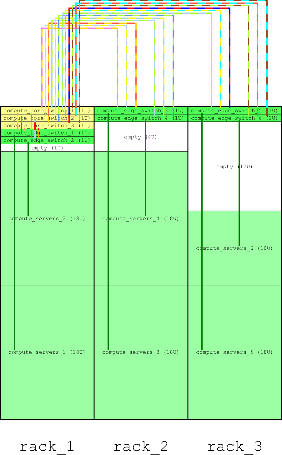
Computer cluster designed by SADDLE, for 100 compute nodes (about 52 TFLOPS of peak performance)
What’s Next?
You can already do a lot with the example database included with SADDLE. Just place proper constraints on the metrics of your compute nodes, choose the number of nodes wisely, and draw conclusions from the designs that SADDLE produces for you. You will certainly find it interesting to observe how economic characteristics of your design change when you change some low-level metrics — for example, choose one type of CPU over another or increase the number of compute nodes.
If you want to add other hardware to the database, edit the XML files. If you want to use SADDLE for your own purposes, feel free to do it — it is distributed under the GPL license.