
The Tool for Automated Design of
Cluster Supercomputers
Disclaimer
This software was created in support of my PhD thesis. Use it at your own risk.
Introduction
The tool can be downloaded here, and will run on both MS Windows and GNU/Linux. The interface is rather intuitive, with lots of annoying pop-up hints — so you will not get lost. Below is an overview of a sample run, to get you started in the minimum time.
(Note: this GUI-based Cluster Design Tool is slightly obsolete. It doesn’t do some advanced stuff, such as placing equipment into racks, calculating floor size or routing cables. For these tasks, please consider using SADDLE that can do all of the above — and more. And yet, the Cluster Design Tool is intuitive and easy to use, allowing you to get a quick introduction into the subject).
The welcome screen
The tool’s window has several tabs, and the first one is called “Nodes”. Building blocks of a cluster supercomputer are compute nodes — individual computers that usually have identical configurations. The “Nodes” tab is used for loading a graph database of compute nodes’ configurations.
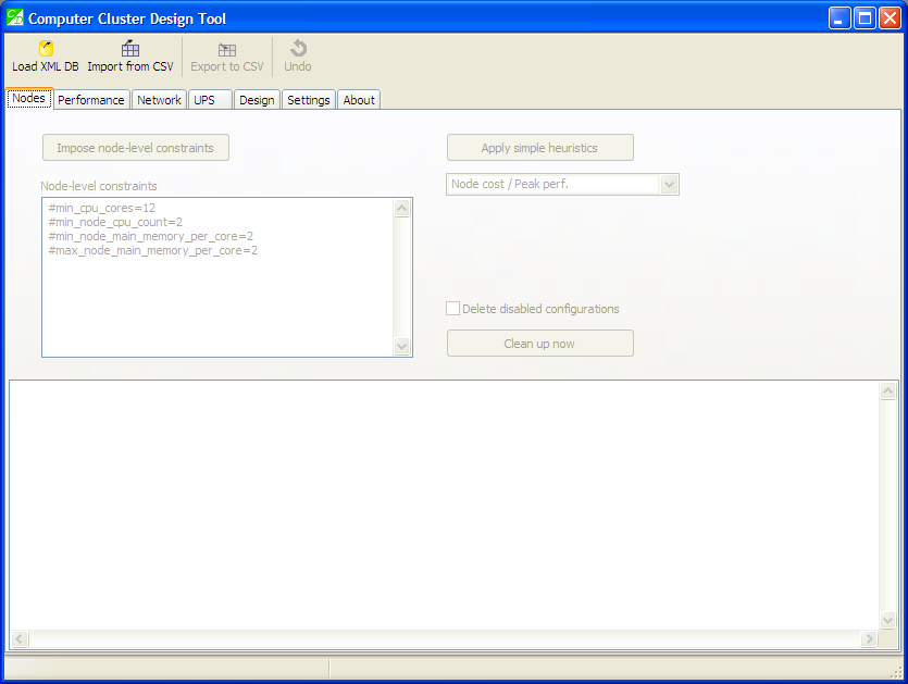
The welcome screen of the tool
Pop-up hints will help you throughout the design process. For example, this pop-up provides comprehensive instructions on using constraints:
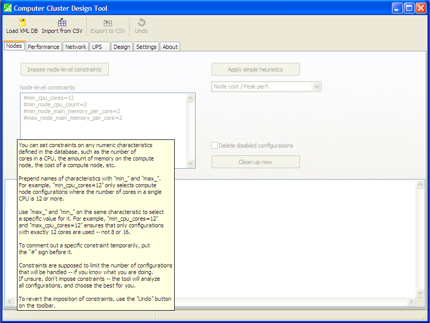
Pop-up hints will help you through the design process
You can load a graph database in its native XML-based format, or alternatively you can import a CSV file that had been previously exported with the “Export” button. Let us load a sample input file, “hp.xml”:
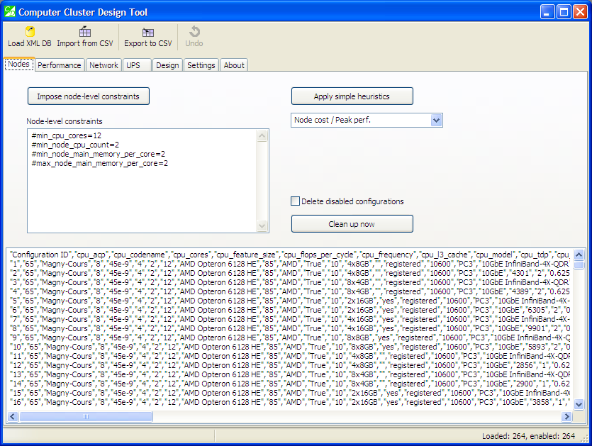
After loading “hp.xml”
After loading the database, the tool identifies 264 configurations of a compute node, computes their technical and economic characteristics, and presents them, in CSV format, in the output pane. You can now export this to a CSV file using the “Export” button — and later import it back, using the “Import” button.
Working with node-level constraints
During the design process, it is not beneficial to perform an exhaustive search. In many cases, you can filter out some configurations of compute nodes by imposing constraints on them.
You can specify node-level constraints in the appropriate pane on the “Nodes” tab. Currently, constraints can be imposed on numerical characteristics of configurations. Choose characteristics whose values you want to limit, prepend their names with “min_”, and specify a minimum value: for example, “min_cpu_cores=12” will allow configurations where the number of cores in a CPU is 12 or more. You can also use “max_” in an analogous way to establish maximum limits: “max_node_cost=4000”.
If you add a comment character # before the constraint, this constraint will be ignored. This is useful if you want to keep the constraint in the pane for applying it at a later time.
Press the “Impose node-level constraints” button to actually impose constraints. Configurations that don’t meet the constraints will be marked as “disabled”, and will not participate in design procedures. You can always see how many configurations are loaded, and how many are still “enabled”, in the status bar.
If you constraints happened to be too strict (too few configurations remained “enabled”), you can revert the action by using the “Undo” button on the tool bar. Try it: impose the constraints and observe in the status bar how many of them remain “enabled”. Simultaneously, the “Undo” button becomes accessible. Press it to revert the action.
You should impose constraints only when you know what you are doing. Otherwise, you can accidentally disable good configurations, thus “throwing the baby out with the bath water”. It may seem that the best configuration of a compute node is the one with the biggest number of cores, or with the highest core frequency, or with the lowest cost — but it is not that easy: if it was, there would be no need for a tool like ours.
Note that imposition of constraints works in the same manner as in the “dbcli” tool.
Applying heuristics
Another way of filtering out configurations is by applying heuristics. It works automatically.
Currently, one heuristic is implemented: “Node cost / Peak performance”. That is, for every configuration of a compute node, we calculate the ratio of the node’s cost to its peak performance, in GFlops. Then, we sort configurations according to this metric (the lower the value, the better), and leave the best 20% of this list. The remaining 80% of configurations are marked as “disabled”.
This heuristic, “Node cost / Peak performance”, tries to approximate the more complex metric, “Total cost of ownership / Real-life performance”, that we make the case for in our framework.
As everything that works automatically and “cuts the corners”, heuristics have some drawbacks. For example, a compute node can have a built-in Gigabit Ethernet adaptor. Optionally, an InfiniBand adaptor can also be installed in addition to the Gigabit Ethernet. Therefore, we would have in our database two configurations: (a) InfiniBand + GigE adaptors, and (b) GigE adaptor only. Both configurations will have the same peak performance, but the former is more expensive than the latter.
As a result, the heuristic would favour the configuration with a Gigabit Ethernet adaptor only, and strike out the configuration with both adaptors. But in real-life settings InfiniBand-connected clusters have higher performance. Morale: heuristics are quick and work automatically, but don’t always produce desired results. If you have plenty of time, try exhaustive search.
Cleaning up the list
After imposing constraints or applying heuristics, many configurations become marked as “disabled” and, although they do not participate in further design procedures, they still take up space in the list, which is visually distracting.
There are two methods to clean up the list. The “Clean up now” button performs a one-time action: it deletes configurations marked as “disabled”, and allows to revert the action via the “Undo” button.
The “Delete disabled configurations” check-box acts differently: as soon as any action is detected that leads to “disabled” configurations (such as application of heuristics or constraints), such configurations are immediately deleted from the list.
Note, however, that one of the actions that leads to “disabled” configuration is the design process itself. In this case, unsuitable configurations will be automatically deleted after the design process is complete, and you will not know why. Therefore, it is recommended to unset the check-box after you have successfully imposed your constraints and applied your heuristics.
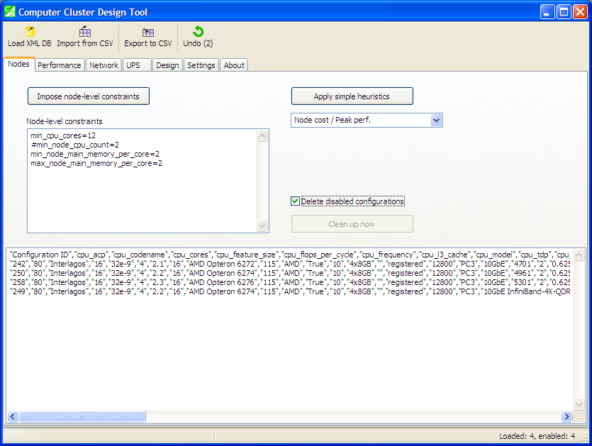
After constraints were imposed and a heuristic was applied, the list shrank to only four positions. The check-box ensures that disabled configurations are automatically deleted. The “Undo” button allows to reverse the actions.
Web services
The core idea of the cluster design tool is that essential parts of the cluster supercomputer can be most efficiently designed by querying web services — small software modules available over network. Each web service has its own “area of expertise”.
This version of the cluster design tool uses the following web services: the “ANSYS Fluent 13” performance model, fat-tree and torus network design module, and UPS sizing module.
The use of web services makes the tool more versatile and future-proof. It is assumed that vendors will be able to host their own web services which, when queried by the tool, will provide the most recent data, such as current equipment prices.
This way, when new products emerge on the HPC market, it will only be necessary to change query URLs.
“Performance” tab
When you open the “Performance” tab for the first time, it has the following elements:
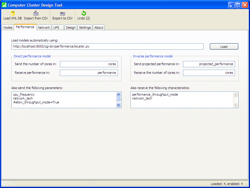
“Performance” tab in its initial state
The first input field contains a URL of a script that will return the list of performance models in “Name=URL” pairs, specifying how each model should be queried. There is no need to be concerned with these details unless you plan to design your own web services for use with this tool.
DetailsThe fields on the screenshot indicate what characteristics of the compute node configuration we should send to the web service, and what parts of the reply we should embed back into the configuration.
With performance modelling, there are two distinct cases: direct and inverse models. Inverse models ask for projected performance, and return the number of cores required to achieve that performance. Direct models do the opposite: they ask for the number of cores, and return the attainable performance.
In this example with “Performance” tab, we send to the web service — the performance model — the following characteristics from the configuration: “projected_performance” (for inverse modelling), “cores” (for direct modelling), and also “cpu_frequency” and “network_tech” (in both cases).
We receive back from the performance model: “cores” (for inverse modelling), “performance” (for direct modelling), and also “performance_throughput_mode” and “network_tech” (in both cases).
The reason that we send “network_tech” and then subsequently receive it back is that the performance model changes it before returning: if several network technologies were available in the compute node configuration, the performance model will choose the best one, and return it.
There is another trick with the “Also receive” field (for all types of web services, not just performance models). Normally, the characteristic indicated here will be searched for in web service’s output, and if found, will be embedded together with its value back into configuration. However, if you specify the value explicitly, such as “my_metric=value”, this will override web service’s output.
The interesting part happens when you press the “Load” button to load the list of models:
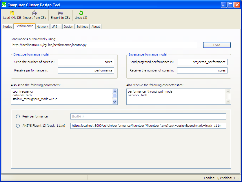
Performance models have been loaded
Now you can choose one of the models that you will use to design your cluster supercomputer. The “Peak performance” model is marked as “built-in”, while the “ANSYS Fluent 13” model has an associated URL which will be queried during the design process.
“Network” tab
The “Network” tab is optional, therefore you can design cluster supercomputers without a network — but this doesn’t make much sense.
The web service used here is the fat-tree and torus design tool. After loading the list of network models, the tool’s window looks like this:
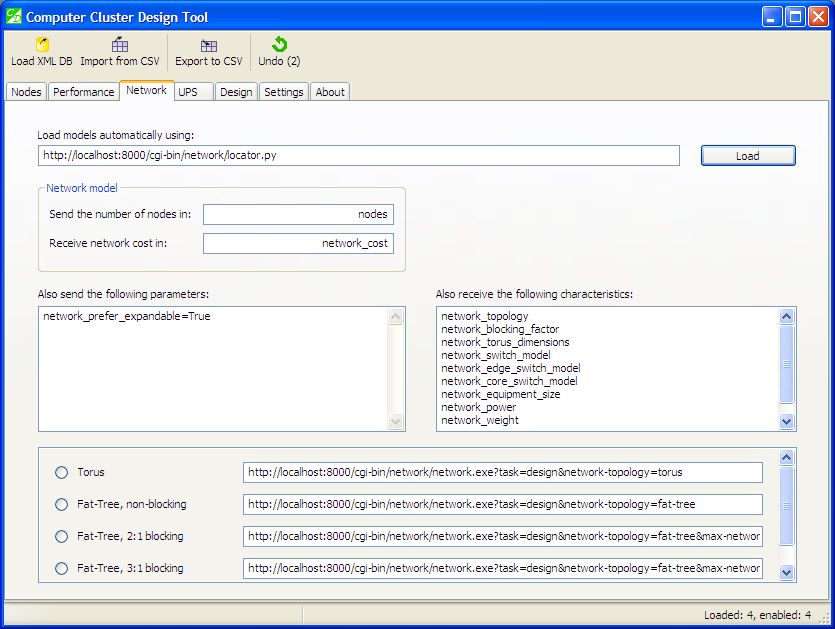
Network models
Here you can choose your preferred topology: torus or fat-tree, the latter being non-blocking or blocking. Select one option.
“UPS” tab
This tab is also optional. The web service used here is the UPS sizing module. After loading the list of models, the window looks like shown below:
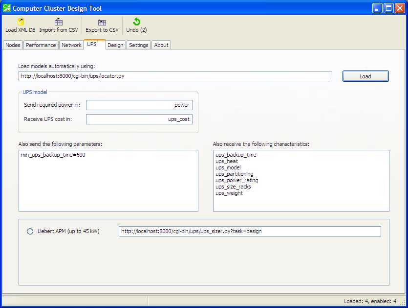
UPS models
Note how we specify here the minimum UPS backup time, in seconds: “min_ups_backup_time=600”. This instructs the UPS sizing module to only select configurations of the UPS system that conform to this constraint.
If we didn’t specify this additional requirement, the UPS sizing module would try to find the cheapest UPS configuration — capable of providing required power but without any specific backup time requirements.
“Design” tab
The most valuable tab of the tool. It is here where you specify global design constraints and objective function.
We refer to the constraints as “global” to differentiate them from the node-level constraints that you can impose on configurations of compute nodes before any design procedures commence. Let’s take a look at the screenshot:
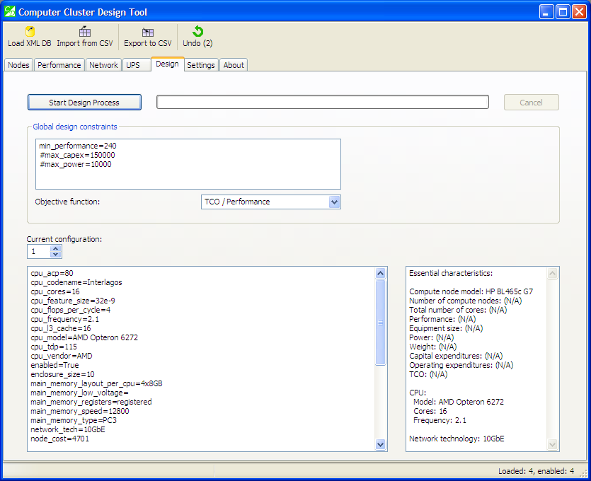
“Design” tab, the most valuable tab of the tool
Note the pane of global constraints. Most of them are optional, except one: “min_performance”. You must specify it. It acts like a foundation stone on which everything else builds.
Also note that units of measurement of this minimum performance are dependent on the performance model that you are using. For the “ANSYS Fluent 13” model, it is measured in tasks per day. For the peak performance, it is in GFlops. Therefore, be careful when specifying it.
Next thing of interest is the objective function. The value of this function will be calculated for each configuration, and then the list will be sorted by this value in ascending order.
Two objective functions are implemented: “Total cost of ownership / Performance” and “Capital expenditures / Performance”. The latter is more of scientific interest; it follows the former closely, but there could be subtle differences. For example, a configuration could be relatively cheap when you buy it, but operating expenditures (energy costs, staff and software licenses) make it expensive in the long run.
The lower part of the window displays a single configuration in “characteristic=value” pairs. This list can be quite long, therefore some essential characteristics are extracted from the list and presented on the right side for your convenience. Many of them are currently marked as “Not available”, because, indeed, they will become available only after the design process completes.
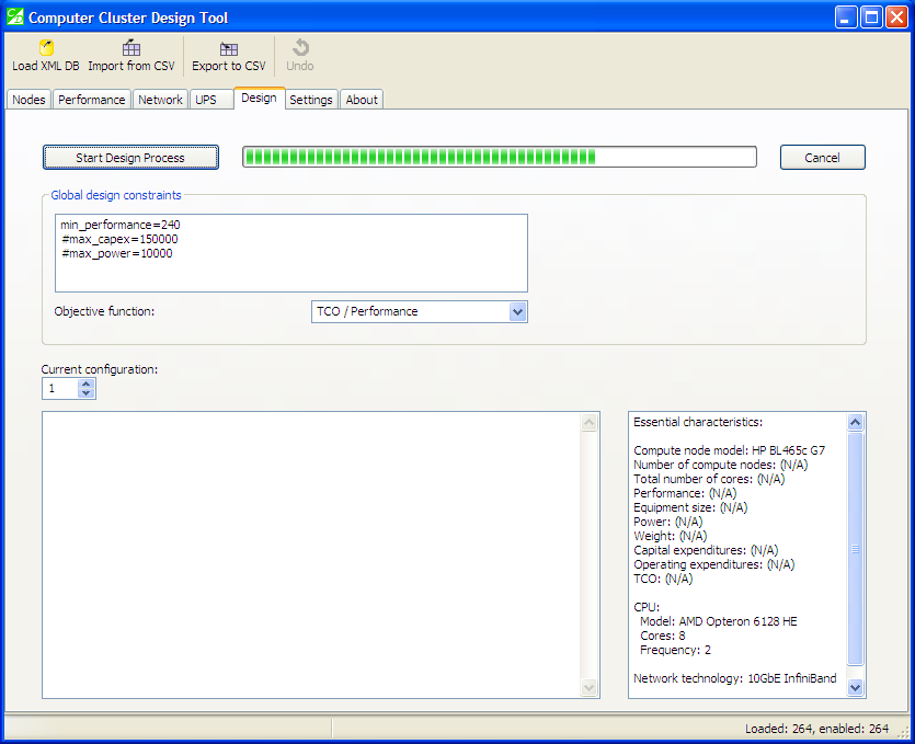
Design procedure in progress. You can cancel it at any time.
“Settings” tab
This tab contains program settings, currently it includes settings that affect operating costs:
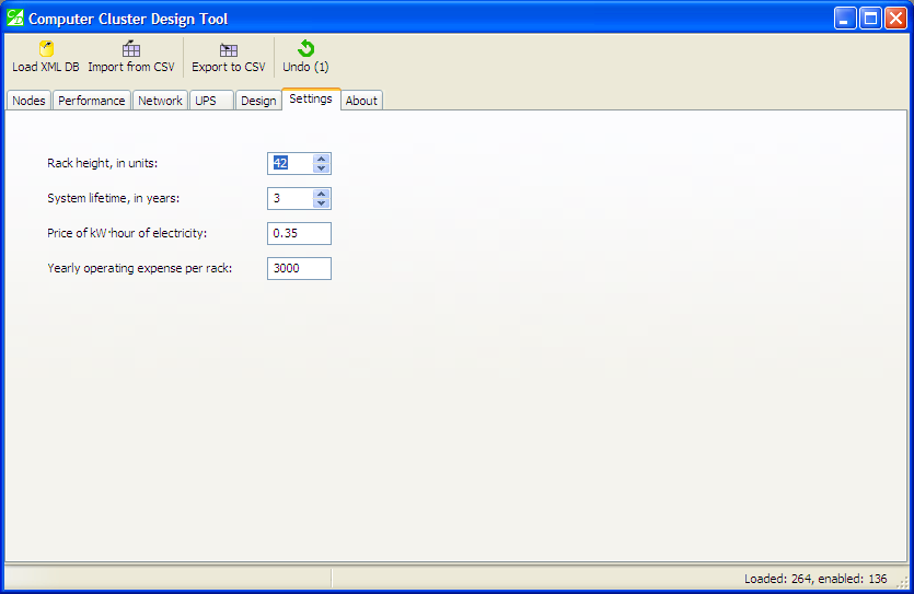
“Settings” tab
Calculating operating costs allows to calculate the total cost of ownership. The settings have reasonable defaults, but feel free to provide your own data. In particular, you may wish to specify electricity price as this figure tends to vary greatly between countries.
The yearly operating expense per rack refers to renting data centre space for housing your racks, with power costs not included.
What happens during the design process?
In accordance with the framework, we do the following actions:
1. Choose the number of compute nodes to attain the minimum performance specified by the user.
2. Design a network with a specified topology to connect those compute nodes.
3. Choose a UPS system that would provide enough power to the computing equipment.
4. Calculate all technical and economic characteristics.
5. Check if global constraints are still met. If not, disable the configuration.
As usual, it appears simple after it has been explained.
Analysing the results
After design procedures are completed, configurations are sorted by the value of the objective function. In the screenshot below, we ran the tool with the following options:
1. No node-level constraints or heuristics (i.e., all 264 configurations will be analysed).
2. Performance model: ANSYS Fluent 13.
3. Network model: Fat-tree, non-blocking.
4. UPS model: Liebert APM (up to 45 kW), “min_ups_backup_time=600”.
5. Minimum performance: “min_performance=240” (for our performance model, this means 240 tasks per day, or 10 tasks per hour).
6. No other global constraints.
You can see in the status bar that out of 264 configurations, only 136 are still “enabled”, which means they passed all checks and meet the constraints:
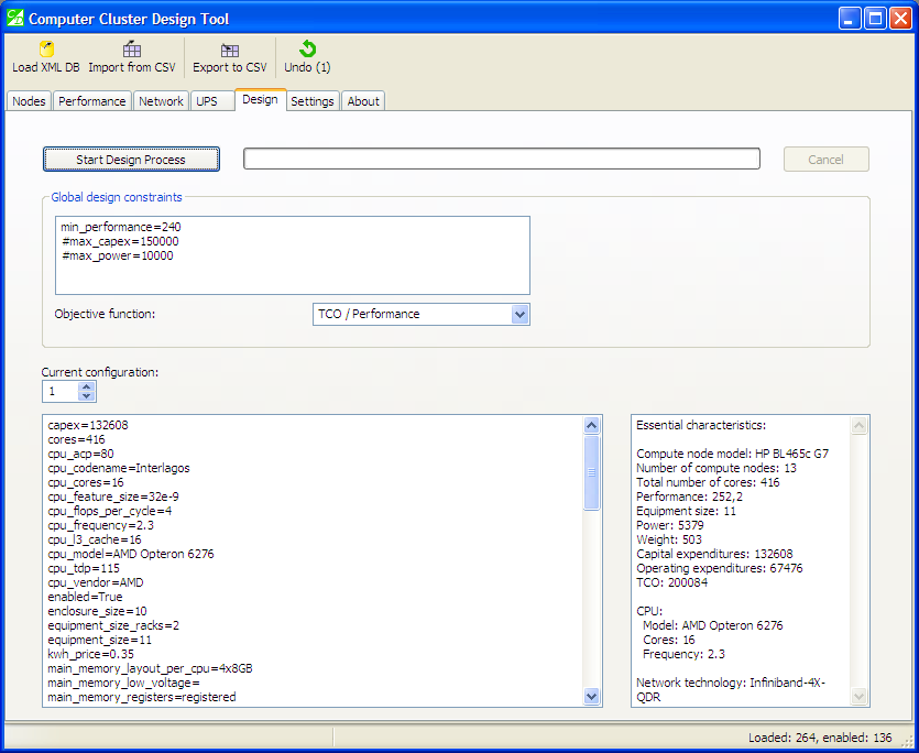
Configurations are sorted by value of the objective function.
The first configuration is the best one — it has the lowest value of the objective function. The pane with essential characteristics lists the performance value of “252,2”. Capital expenditures for this configuration are 132,788 (US dollars).
The worst configuration that still meets the constraints — number 136 — has capital expenditures of 514,558 US dollars — almost four times higher. (Further investigation shows it uses outdated CPUs with a low clock frequency).
All other configurations — and all of them use 10Gbit Ethernet network adaptors — cannot attain the required performance of 240 tasks per day. This happens because no matter how many compute nodes we connects with a high-latency 10 Gbit Ethernet network, the overall performance “flattens out”, and never reaches the required rating of 240 tasks per day. See a more detailed explanation on the ANSYS Fluent performance model page.
It is worth noting, however, that some of the 10 Gbit Ethernet configurations still can attain 240 tasks per day. This requires a large number of compute nodes with high-frequency CPUs. Power consumption of those configurations was on the order of 10kW, compared with only 5,3kW for the optimal configuration. Therefore, if constraints on power or equipment space were specified, these configurations would be filtered out.
Why configurations become “disabled”
If a configuration is disabled, you will see a big red dot above it. Hover your mouse pointer over the dot, and a hint will pop up, telling why exactly this configuration was “disabled”:
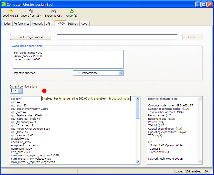
For disabled configurations, hover the mouse pointer to learn why it was disabled.
This particular configuration was disabled due to the reason discussed above: performance “flattens out” with high-latency network, and the so-called “throughput mode” is required to run 240 tasks per day. Other reasons why configurations become disabled include node-level constraints and heuristics.
Yet another reason is the inability to construct a fat-tree network for a very large cluster supercomputer: this happens because two-level fat-trees that our web service designs can only accommodate a limited number of compute nodes that depends on the choice of network switches. If this is an issue for you, edit the database of the network design module and add switches with a high number of ports.
Why some constraints could not be tested?
Besides the red dot mentioned in the previous section, you can sometimes encounter its sister, the yellow dot. The yellow dot means that some constraints for this configuration could not be tested. Therefore, the configuration might be suitable, but this could not be automatically verified.
There are two possible scenarios as to how the yellow dot can appear:
1. Yellow dot appears by itself.
The reason is that you specified some global design constraints that could not be checked for the current configuration because their values were not available. The most common reason is that a web service failed to return them. For example, if you specified the following global constraint: “network_equipment_size=10” to limit the size of network equipment to 10 rack-mount units, but the web service that you used to design networks didn’t return this metric, then the constraint could not be checked, and the yellow dot will appear.
Remember that you can control what metrics web services return by using the “Also receive the following characteristics” pane of the respective web service. If the web service doesn’t know how to calculate the metric that you need for your design purposes, contact the vendor: in case of network design web service, contact the network hardware vendor, etc.
2. Yellow dot appears alongside the red dot.
This usually happens when you specified perfectly reasonable constraints, but the configuration was disabled (hence the red dot) before the relevant metric was calculated, and constraint could be checked. For example, if during the design process the tool detects that the cost of compute nodes exceeds the available budget (specified with “max_capex” constraint), then the configuration is immediately disabled, and no further design procedures are run: no network is designed, no UPS system is chosen, etc. Therefore, the red dot indicates that the configuration was disabled, and the yellow dot indicates that it was disabled too early in the process, when the constraints could not be checked yet.
Sample output
Here is the sample output of this run, in CSV format: sample_output.csv. You can open it in your favourite spreadsheet (I prefer Apache OpenOffice).
What next?
You can run your own copy of the tool and web services by downloading them.
Questions? Comments? Please leave your feedback below.