Learn how to design fat-tree networks and use our simple tool for designing your own interconnection networks!

1. See also: my articles on designing fat-tree and torus networks.

2. For fat-tree networks built with Ethernet hardware, check this

The tool demonstrates the process of designing cost-efficient two-level fat-tree networks for your cluster supercomputers. Please read the following “Fat-trees Primer” before using the tool. It provides an introduction to the method and the algorithm used by the tool.

I am brave and bold, get me right to the tool!

 

Teach Yourself Fat-Tree Design in 60 Minutes

Introduction

In a switched fabric — a network topology that uses switches — the main goal is to connect a large number of endpoints (processors or servers) by using switches that only have a limited number of ports. By cleverly connecting switching elements and forming a topology, a network can interconnect an impressive amount of endpoints.

Fat-Tree networks were proposed by Charles E. Leiserson in 1985. Such network is a tree, and processors are connected to the bottom layer. The distinctive feature of a fat-tree is that for any switch, the number of links going down to its siblings is equal to the number of links going up to its parent in the upper level. Therefore, the links get “fatter” towards the top of the tree, and switch in the root of the tree has most links compared to any other switch below it:

Fig. 1. Fat-Tree. Circles represent switches, and squares at the bottom are endpoints.

This set-up is particularly useful for networks-on-chip. However, for enterprise networks that connect servers, commodity (off-the-shelf) switches are used, and they have a fixed number of ports. Hence, the design in Fig. 1, where the number of ports varies from switch to switch, is not very usable. Therefore, alternative topologies were proposed that can efficiently utilise existing switches with their fixed number of ports.

There is a controversy whether such topologies should be called fat-trees, or rather “(folded) Clos networks”, or anything else. However, the term fat-tree is widely used to describe such topologies. The example of this topology is given below:

Fig. 2. Two-level fat-tree network. The network is built with 36-port switches on both levels. A total of 60 nodes are currently connected.

Here, a two-level fat-tree network is depicted. The lower and upper levels can be referred to as edge and core layers, respectively. Identical switches with 36 ports are used on both levels. Each of the four switches on the edge level has 18 ports dedicated to connecting servers (the small circles in the bottom of the picture). The other 18 ports of each edge switch are connected to the core layer. In this case, two bundles of 9 links (represented by thick lines) go to the two core switches.

Exercise. Find the rightmost edge switch. How many ports does it have connected to the core level? How many ports are currently connected to the servers?    Spoiler: (18 ports are connected to the core level: nine are used by “green” links that go to the 1st core switch, another nine are occupied by “cyan” links that go to the 2nd core switch. As for the servers, currently six are connected, with the possibility for expansion by 12 more servers)

If two servers connected to the same edge switch wish to communicate, they can do so via that particular edge switch, without referring to the core level. If, on the contrary, the servers are connected to different edge switches, the packets will travel up to any of the core switches and then down to the target edge switch.

Exercise. Which paths are available for packets travelling from first to second edge switches?    Spoiler: (The “green” path through the 1st core switch, and the “cyan” path through the 2nd core switch, for a total of two paths)

As you can see, every edge switch maintains the distinctive property of the original fat-tree network: the number of links that go to its siblings (the servers) is equal to the number of links that go to its parents. The difference with the original fat-tree is that the intermediate switch has several parents (in this case, two), whereas in Fig. 1 each switch only has one parent. That is the source of controversy in terminology described above.

Such topologies (we will still call them fat-trees) are widely employed in cluster supercomputers, usually using InfiniBand network technology as their foundation (for Ethernet-based fat-trees, click here).

How many nodes could you have in a network?

If edge switches have Pe ports, and core switches have Pc ports, then the largest two-level fat-tree that can be built will connect Nmax=Pe*Pc/2 servers (smaller trees can also be built if necessary). Suppose we use one of the biggest currently produced commodity switch with P=648 ports, and employ the same switch model on both edge and core levels (Pe=Pc=P), then Nmax=P*P/2=648*648/2=209,952. This is more than enough for many supercomputers! If even more servers need to be connected, a three-level topology can be built.

Exercise. How many nodes will have the largest two-level fat-tree that you can build using 36-port switches?    Spoiler: (Nmax=36*36/2=648 nodes)

For every additional level that you add to your network, you multiply the number of nodes by P/2. Therefore, a three-level network can connect Nmax=P*(P/2)*(P/2)=2*(P/2)³ nodes, and for L layers Nmax=2*(P/2)^L nodes.

However, many cluster supercomputers only have on the order of several thousands compute nodes, and that is where variety comes into effect: you could use many small switches for your design, or a few large ones instead. There are many possible variants that would differ in their cost, possibility for future expansion, volume of equipment (how much space it takes in racks), power consumption and other important characteristics.

In fact, there are more variants that human designers tend to consider. Hence, it is beneficial to use a tool that automates the design process of fat-trees.

Blocking

We noted above the property of fat-tree networks in their primary meaning: on each intermediate level, the number of links that go to the upper level (in two-level networks, this is from the edge level to the core level) is equal to the number of links going to the lower level (here, from the edge level down to nodes). On this intermediate switch, the number of uplinks and downlinks are in proportion of 1:1. Such networks are called non-blocking. You can arbitrarily divide nodes into pairs, and if all pairs start communicating, still every pair of nodes will be able to communicate at full link bandwidth.

For circuit-switching networks, you could designate a separate path between all communicating pairs, and there would be enough paths for every pair. In packet-switching networks that we consider here the same non-blocking effect is maintained in a statistical sense.

You can distribute downlink and uplink ports in a different proportion. For example, you could have twice more ports going down than going up (2:1), which is a blocking factor of 2. For 36-port switches, this means 24 ports going down and 12 ports going up. You could also have, say, 2,6:1 or 4:1 blocking. The sum of ports would still be 36, only the distribution would change.

Exercise. To which port distribution does a blocking factor of 2,6 correspond? Spoiler: (26 downlinks and 10 uplinks. The sum is still 36)

Exercise. What is the biggest possible blocking factor when using 36-port switches? Spoiler: (Of 36 ports, 35 can be dedicated to downlinks, and one to an uplink. Therefore, the blocking factor is 35)

For packet-switching networks, having a blocking network means that two packets that would otherwise follow separate paths, would be queued and one of them would have to wait. This introduces latency which is never good for parallel computing.

Blocking is only used because it allows to make somewhat cheaper networks: fewer switches are necessary. However, as the blocking factor keeps increasing, the cost of network doesn’t proportionally decrease. The other alternative use case for blocking networks is to connect more nodes using the same hardware than a non-blocking network can sustain.

With a blocking factor of Bl, an edge switch has Pe*Bl/(Bl+1) downlinks. In the non-blocking network, Bl=1, hence an edge switch has Pe/2 downlinks. Therefore, with a blocking factor of Bl, a network can sustain 2*Bl/(Bl+1) times more nodes, which is less than two for any blocking factor (even with a high blocking factor of Bl=2,6 you can connect only 44% more servers).

Blocking limits performance. Different parallel applications demonstrate different slowdowns when blocking is imposed. Some of them are more “forgiving”, and some are less. Although the cost of your supercomputer decreases when using blocking, the performance often decreases faster. See references in the end of this tutorial for two papers that discuss performance effects in different blocking scenarios.

What switches are available?

Commodity hardware is widely used for cluster supercomputing, because economy of scale ensures considerable reduction of cost per unit for all types of equipment.

The current (February 2012) de-facto standard for InfiniBand equipment is 4X QDR InfiniBand. (Update from November 2012: FDR is now the standard). Perhaps the simplest model of InfiniBand switch currently produced is the “monolithic” (or “fixed configuration” — i.e., not modular) 36-port switch. It takes one unit of rack space, and its main panel has 36 ports. Such a switch has a chip inside — an integrated circuit — that is capable of handling packet flows from exactly 36 ports. Remember that you can connect a fairly large number of nodes by using just 36-port switches and building a fat-tree with them.

However, if you need more nodes in your cluster, you have to use something different. Here is where the modular switches come in handy. A modular switch consists of a chassis (a metal frame) where modules can be installed. Power and management modules are the example of infrastructural modules; both types can be redundant for greater fault tolerance.

But most important for your networking tasks are fabric boards and line boards. As a matter of fact, modular switches are themselves two-level fat-trees, only combined in a single box. Fabric boards, also known as spine modules, are in effect core-level switches, while line boards, also called leaf modules, are edge-level switches. They use the same chips (e.g., with P=36 ports) as the “monolithic” switches.

Exercise. Suppose you use 648-port modular switches on both core and edge levels to build your fat-tree. But such switches already implement a two-layer fat-tree internally. Hence, if you cascade them, you essentially receive a four-level fat-tree. Using the formula for Nmax from the above material, calculate the number of nodes that a four-layer network can support when using chips with P=36 ports. Compare this to a direct calculation of Nmax for a two-layer network with P=648 ports. Spoiler: (In the general case, Nmax=2*(P/2)^L. With L=4 layers and P=36 ports, this yields Nmax=2*(18^4)=209,952 nodes. If we consider switches as big black boxes with P=648 ports, then Nmax=648*648/2=209,952. This is the same result, but obtained with a lower level of details)

It is required to install all fabric boards into the modular switch to make it non-blocking — so that each node can communicate with every other node without congestion. If you know that your application has modest bandwidth requirements, you can save some money by not installing some fabric boards, effectively making the switch blocking. However, network cost constitutes only a small share of the cost of your entire cluster computer, so such savings will not really pay off.

Resistance to failure

Fabric boards are “redundant” per se: if one of them stops functioning, the other boards will still carry traffic, hence the network will run in a degraded mode (with blocking); however, all nodes will still be reachable.

Exercise. Refer to Fig. 2. Perform a thought experiment: remove one of the core switches and links that originate from it and proceed down to edge switches. Ensure that any server still can reach any other server, using the remaining core switch.

Line boards are another matter. They act as edge switches: their “outer” side is visible as ports on the modular switch’s panel, while its “back” side is connected to fabric boards inside the modular switch. The number of line boards you need to install is proportional to the number of ports you want to have in your switch.

Also, if a line board fails, then all nodes connected to its ports will be unable to communicate. If you really require the ultimate level of fault tolerance, you could equip your compute nodes with dual network interfaces, and connect each of them to separate switches (or at least to separate line boards, if you only have one switch). This is sometimes referred to as “dual-plane connection”. This can also be used to provide more bandwidth for compute nodes, which is especially helpful when using modern multicore CPUs in compute nodes.

Exercise. Again, refer to Fig. 2. Pick up an edge switch of your choice and remove it, together with the links that go down to servers and links going up to the core switches. Ensure that the servers that were connected to this switch become isolated and are now unable to communicate both with each other and with the rest of the fabric. Were these servers simultaneously connected to a different edge switch (read: line board of a modular switch), they would have retained connectivity.

Another disaster that can occur in two-level networks is the loss of connectivity between an edge switch and one or several (or all) core switches. If some core switches are still reachable from a particular edge switch, this network segment runs in degraded mode as described above. If all core switches are unreachable, this network segment becomes isolated from the rest of the fabric, although servers connected to this particular edge switch continue to communicate (unfortunately, for most applications this doesn’t help much).

This type of malfunctioning can happen because of cabling issues, and can affect “hand-made” two-level fat-trees. Modular switches, albeit they implement a two-level fat-tree internally, have a much more reliable connection between line and fabric boards inside the chassis. So, if your two-level network is implemented inside a single switch, you can safely ignore such a problem.

An example of a modular switch

A good example of a modular switch is a 144-port model. It accommodates up to 4 fabric boards (remember, these are used for delivering throughput, by introducing several possible paths between edge switches), and up to 9 line boards. Each line board has 18 ports, but if you want to have a fully non-blocking fabric (where all possible pairs of nodes can simultaneously communicate at full speed), then you shall only use 16 ports out of 18. As discussed above, some HPC applications are “forgiving”, and allow for this small blocking.

A modular switch occupies the same amount of rack space irrespective of how many line boards are fitted into the chassis. Even the minimal configuration with only one line board installed will cost a hefty sum, because the cost of chassis, infrastructural modules (power and management) and fabric boards cannot be reduced. Therefore, modular switches usually become profitable when they are populated fully, or close to that.

Even in the fully populated modular switch, the cost per port is 3 to 4 times higher than in a “monolithic” switch. However, modular switches provide opportunities for easy expansion. Also, when the cost of compute nodes is taken into account, the cost per connected server does not differ that much.

Technical characteristics of switches

After a series of corporate mergers and acquisitions, we now have two major manufacturers of InfiniBand switches: Mellanox Technologies (which acquired Voltaire in 2010) and Intel (which acquired QLogic in 2012).

Many different models of modular switches are sold on the market, from a 96-port model occupying 5U of rack space (by QLogic) and 108 ports in 6U (by Mellanox), to 648 nodes in 29U (by Mellanox), to 864 ports in 29U (by QLogic).

Switches are characterised by a number of metrics, with the most important being the number of ports, size they take up in the rack, power consumption (which immediately translates into cooling requirements), and, of course, cost. If you divide size, power and cost by the number of ports, you will receive per-port metrics.

Similarly, if a network is built using a number of (possibly different) switches, it will also be characterised by size, power and cost. These metrics are additive: the cost or size of a network is given by the sum of costs and sizes of switches that comprise it.

Exercise. In Fig. 2, the switches typically consume 106W (with copper cables). With 70 servers, how many watts does the network require on average in order to connect one server? Spoiler: (There are 6 switches in the network, which together consume 6*106=636W. That is 636/70=9.08W, or approximately 9W per each of 70 servers)

Exercise. If you didn’t need to provide full non-blocking connectivity between the 70 compute nodes, how many of the above 36-port switches would you need, then? How many times would you reduce power consumption, size of equipment and costs? Spoiler: (To connect 70 nodes using 36-port switches, you would plug 35 of them into the first switch, and the remaining 35 into the second one. Finally, you would connect two switches together using their 36th ports. In total, you would need 2 switches instead of 6. This reduces everything — cost, size, power — three-fold)

Designing your network

Trivial case: the star topology

Let’s get to the most interesting part, the design process itself. We’ll start with three trivial cases. The first one refers to the star topology of your network — when you can avoid building a fat-tree (because someone else implicitly does it for you).

Now you know that you can build a 648-port network using just 36-port switches, but would it be really useful? Because this way you would have 54 switches in total. Instead, you could buy a single 648-port switch (which also implements a two-level fat-tree internally). One big switch is easier to manage than 54 small switches. The wiring pattern is really simple: you just place the switch in the geometric centre of your machine room, and draw the cables from every rack to it. Any cabling between the edge and core levels is now inside the switch and is therefore very reliable (and you also save on cables!)

Also, if you plan to initially have, say, 300 nodes in your cluster, then the modular switch is easier to expand: you just add required line boards. With the “hand-made” fat-tree network, you would have to carefully design the core level to be big enough to accommodate future expansion; otherwise you would need to rewire many cables, which is error-prone and costly.

So, if your cluster is small enough to use a single switch, then perhaps the star topology is the way to go. The biggest InfiniBand switch produced so far is probably the famous “Sun Data Center Switch 3456”, with 3456 ports of the now outdated 4X DDR technology. But modern switches up to 864 ports are available on the market, so smaller clusters can be built using star topology.

Using a single big switch is more expensive than building the same network manually with smaller switches, but convenience, expandability and manageability considerations all suggest to follow this path.

Just two edge switches

Sometimes, if you try to build a fat-tree network for a small number of hosts using the formulae below (or the tool, which uses the same formulae), you can arrive to a situation when you are offered to use two edge switches and one core switch. This is a degenerate form of a fat-tree network, and you can further simplify it by getting rid of the core switch and simply connecting the two edge switches to each other using all their available ports. Throwing out the core switch will reduce both costs and latency.

An unusual star network: two blade server chassis

There is yet another case when you don’t need to implement a fat-tree. This is the case of exactly two blade server chassis. The chassis, also called “enclosure”, is a metal frame where blade servers are inserted. The chassis has compartments to house switches, including InfiniBand switches. In our terms, these are essentially “edge” switches. Upon insertion of an InfiniBand switch, blade servers become electrically connected to its “internal” ports. The other half of the ports of this edge switch are implemented as usual InfiniBand connectors accessible from the rear side of the chassis.

So, if you have exactly two chassis with blade servers, then you don’t need to build a fat-tree. You can just connect two chassis together using a bunch of cables, like mentioned in the previous section on two edge switches. But there is more. In fact, you don’t need two switches in this case. Instead of one of the switches, you can install a so-called “pass-thru module” (if your vendor supports it).

The “pass-thru module” is a fancy device that relays signals from your blade servers to the usual InfiniBand connectors on its rear side. It looks similarly to the InfiniBand switch intended for blade chassis, but the difference from the switch is that it does not switch packets between your servers. Rather, the pass-thru module must be connected to a real, bigger switch. If two servers inside your chassis want to communicate, they cannot do so with a pass-thru module: the packets will have to exit the module and chassis, and enter a real switch. The main purpose of the pass-thru module is cost reduction: it costs an order of magnitude less than a usual blade switch.

This way, you have chassis A with a real switch inside, and chassis B with a pass-thru module, and as many cables between the chassis as there are ports on the blade switch in chassis A. Physically, this looks as two items of equipment. But logically, this is still the old good star network topology. Indeed, there is only one switch — the one in chassis A. Blade servers in chassis A connect to it using internal PCB connector inside the chassis. Blade servers in chassis B connect to it using cables. With a bit of imagination, you will recognise a star network in it.

Building the edge level

So, let us suppose that the trivial cases of star network are not for you. Either your cluster has more ports than the biggest switch available on the market, or you use blade servers and want to utilise more than two chassis. Then, you need to build a fat-tree. This paragraph concerns building the edge level.

On the edge level, everything is rather simple. Proceeding from the desired blocking factor (or using Bl=1 for non-blocking networks), you first calculate how many ports on edge switches will be connected to nodes. Let’s denote this as Eptn — “edge ports to nodes”. The remaining ports on edge switches can be used as uplinks. We will denote this as Eptc — “edge ports to core”:

Eptn=Trunc (Pe * Bl / (1+Bl))
Eptc=Pe – Eptn

Here, “Trunc” is the truncation function. Its use ensures that you don’t accidentally design a network with blocking bigger than requested. For example, if blocking of 4 is requested and Pe=36, the above formula would give Eptn=28. The remaining Eptc=36-28=8 ports would be used as uplinks. The resultant blocking factor is therefore 28/8=3,5. If we used 29 downlink ports, the blocking would be 29/7=4,14, which is higher than was requested.

Now we can calculate how many edge switches are required:

E=Ceil (N / Eptn)

(“Ceil” denotes the ceiling function, it returns the nearest integer number bigger or equal to its argument).

Exercise. How many 36-port edge switches would you need to connect 70 nodes in a non-blocking scenario? 72 nodes? 74 nodes? Spoiler: (In a non-blocking scenario, Bl=1, hence Eptn=Pe/2. With N=70, E=Ceil(N/(Pe/2))=Ceil(70/(36/2))=Ceil(70/18)=Ceil(3,88)=4. Therefore, E=4. Refer to the omnipresent Fig. 2 to verify this answer. Same story with N=72. But with N=74, E=Ceil(4,11)=5. You will need 5 switches — one of them will be only slightly utilised. Alternatively, you can uniformly distribute 74 nodes between 4 switches: on two switches you will use 18 ports, and on the other two you will use 19 ports. The blocking factor for the last two switches is 19/17=1,12, which might be acceptable for your applications)

The current industrial “dogma” is to use the smallest “monolithic” switches as edge switches. They are even referred to as “top-of-rack switches”. Today, this means 36-port switches. For example, in a standard 42U rack you can place 2 edge switches (1U each), each serving Pe/2=18 nodes (also 1U each). In total, there would be 38U of equipment. 4U would be available for other uses, or wasted.

In case of blade servers, the edge switches are in your chassis. For example, a blade chassis can contain 16 servers and occupy 10U of rack space. You can place 4 chassis into the rack, for a total of 40U. The edge switches are located inside the compartments of the chassis, and therefore don’t occupy rack space on their own. In this scenario, 2U of the rack space are waisted.

Exercise. Another manufacturer provides blade chassis of 7U height. How much rack space is waisted in this case? Spoiler: (With 7U height, you can install 6 chassis that will occupy exactly 42U of space. No space would be wasted!)

There are situations when 36-port edge switches are not big enough to connect all nodes in your cluster — but they still could be used for 95% of machines in the November 2011 TOP500 list. On the other hand, even though 36-port switches are theoretically usable as edge switches for big machines, modular switches in this role make cabling and maintenance much simpler.

Building the core level

Here is how you build the core level. Take one core switch. For every edge switch, connect its first port to the core switch. As you have E edge switches, you will occupy E ports on your core switch as a result of this operation.

Now, repeat this step several times until you run out of ports on your core switch. If you performed this step for a total of, say, B=4 times, then you would notice that now each of your edge switches is connected to the core switch with a bundle of B=4 links. B can be obtained with a simple equation: B=Pc div E, where Pc is the port count of your core switch.

By now, your core switch has B*E occupied ports, and Pc mod E ports are not used, or waisted. For Fig. 2, B=Pc div E=36 div 4=9. No ports are waisted on core switches, as Pc mod E=0. However, in general, you core switch might have some waisted ports.

The steps above result in the following: each of your edge switches has B ports occupied, and there is one core switch which is completely used. You need to connect remaining ports of your edge switches by installing more core switches in the same manner. How much of them do you need?

There are two possible alternatives. With the first one, you fill ports of edge switches as densely as possible, and the last edge switch usually has some spare ports. After you put your equipment into racks, this scheme allows for easier expansion using those spare ports. In this scenario, you have Eptc ports that need to be connected to the core level, and one core switch gave you B connections. Hence, you need C=Ceil (Eptc/B) core switches.

Example. Connect N=128 nodes, with Pe=Pc=36 ports and a blocking factor Bl=1. Calculate E and C, the number of edge and core switches, respectively.
As Bl=1, Eptn=Eptc=Pe/2=18.
Then, E=Ceil (N/Eptn)=Ceil (7,1)=8.
B=Pc div E=36 div 8=4.
C=Ceil (Eptc/B)=Ceil (18/4)=Ceil (4,5)=5.
The answer is: E=8, C=5.

But there is another alternative that can save you some money: distribute your nodes uniformly among edge switches. In this case, the number of edge ports going to nodes, Eptn, is calculated once again and now equals Eptn=Ceil (N/E). Correspondingly, the number of ports going to the core level is also recalculated, and it equals Eptc=Ceil (Eptn/Bl). B and C are then computed as usual.

Example. Redo the above example, this time trying the uniform distribution of nodes among edge switches. Check if this leads to savings.
We already computed Eptn=Eptc=18, and E=8. If we uniformly distribute nodes among edge switches, then Eptn changes to:
Eptn=Ceil (N/E)=Ceil (128/8)=16.
Correspondingly, Eptc=Ceil (Eptn/Bl)=16. Now, compute B and C as usual:
B=Pc div E=36 div 8=4.
C=Ceil (Eptc/B)=Ceil (16/4)=4.
The answer is: E=8, C=4.

As can be seen, this solution spares one core switch. However, it makes spare ports on edge switches hard to utilise in case expansion is necessary. Indeed, after equipment was densely installed into racks, the only way to use spare ports on edge switches is to install new equipment into new racks and draw long cables from it to the spare ports, in irregular patterns. Compare this to the above variant: all spare ports were located on the last edge switch, which makes them more easily accessible for expansion. As a result, the tool that implements this algorithm chooses uniform distribution only if explicitly directed by the user, or if it decreases the number of core switches. We will also see below how to handle future expansion.

If you need to try different models of edge and core switches, establish nested loops and try them in order (that’s exactly what the tool does).

Let’s review another example for clarity.

Example. N=320, Pe=32, Pc=36, Bl=1. This describes five racks, each with four enclosures, each with 16 blade servers. Eptn=Eptc=16. Here, E=20 — this is as expected, because there are 5*4=20 enclosures, and there is one edge switch in each enclosure. Then, B=Pc div E=1 and C=Ceil (Eptc/B)=16. This is quite an infelicitous configuration, because core switches will each have Pc mod E=16 (almost half!) unused ports. In total, E+C=20+16=36 switches are needed. Redo this example with N=288 nodes and see what changes. Spoiler: (N=288, Pe=32, Pc=36. Hence, E=18, B=2, C=8. In total, E+C=18+8=26 switches are needed)

As you can see, this is fairly easy — at least, after it has been explained. The most mundane task is to set up a loop to try many possible combinations of edge and core switches, and for every combination calculate its technical and economic characteristics.

On the other hand, with blade servers, so popular today, you only have one choice of edge switches — the ones provided by the vendor. So, you don’t need to analyse many hardware combinations. Still, automating the process helps to avoid mistakes.

Dealing with link bundles

When you calculate B, the number of links in a bundle running between edge and core layers, the formula for B gives you the thickest possible bundle size, because one thick bundle is usually more convenient to route than many separate cables.

Remember that your edge switches have Eptc ports that need to be connected to C core switches. The formula for B assumes that cable bundles going to the first C-1 core switches will contain B cables each. On each edge switch, this will utilise B*(C-1) out of Eptc ports that need to be connected to the core level, and the remaining Eptc-B*(C-1) ports will go to the last core switch.

However, sometimes you end up with only two core switches, and the above calculations can produce surprising results. Let’s consider an example. We want to interconnect N=90 nodes using switches with Pe=Pc=24 ports, with the blocking factor Bl=4. On each edge switch Eptn=19 ports will be dedicated to nodes, and the remaining Eptc=5 ports will go to the core level. You will have E=5 edge switches. Calculation of B yields B=Pc div E=24 div 5=4. Then, C=Ceil (Eptc/B)=Ceil (5/4)=2. So, you need to distribute Eptc=5 ports on each edge switch, with bundles of B=4 links, between C=2 core switches. How is this possible?

The trick is that 4 out of Eptc=5 ports will be connected with a bundle of B=4 links to the first core switch, and the remaining fifth port on each edge switch will go to the second core switch. That’s how it looks:

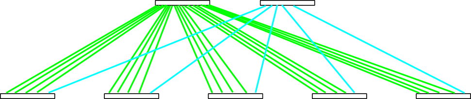Fig. 3. Non-uniform distribution of links among core switches.

This wiring is uneven, and also the two core switches are unevenly loaded with packet processing. Instead, you can distribute links more uniformly: a bundle of 3 links to the first core switch, and a bundle of 2 links to the second:

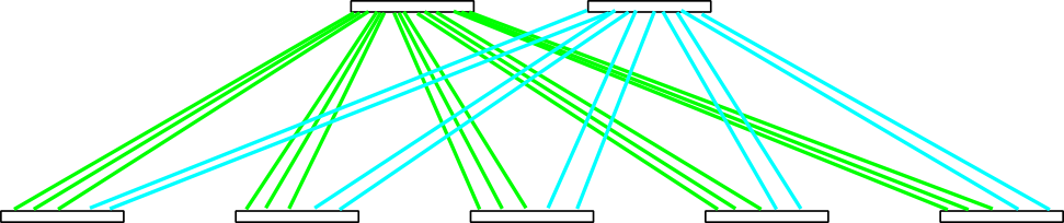Fig. 4. More uniform distribution of links.

(Note with regard to this particular case that in Fig. 3 you could just connect all edge switches to only one core switch: for the blocking factor Bl=4 chosen for this example you need 25 ports, and it has 24, which is almost as good. There are situations when two core switches are still preferable: (a) when you need improved reliability: the second core switch brings reliability through redundancy, and (b) when you are planning future expansion of your network; see the next section, “Designing for expandability”).

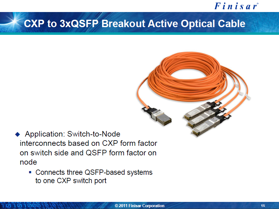
There is one more thing you might want to keep in mind. There are core switches with CXP connectors, and there are cables that “fan out” from one CXP connector to three standard QSFP connectors found on regular InfiniBand devices (see example from Finisar below). This way, if you arrange links in bundles of B=3, you can implement each bundle with this type of cable:

Designing for expandability

When you try to expand your network, you will need more edge switches. But what is worse, sooner or later you will also need more core switches as well. The wiring between the layers is intricate, and if you want to expand your network, you would need to re-wire many connections. This is a costly and error-prone process.

But fortunately, there is a better way to cope with it. You just have to design your core level in such a way that it has enough spare ports to accommodate the largest future expansion.

This means initially procuring and installing more core switches than you would in a non-expandable network, and having a low core level port utilization. Edge switches, however, are procured in just the proper amounts, and are not reserved for future use. For every stage of expansion, more edge switches can be added. The existing cabling will not require rewiring; only new cables will need to be laid.

Let us give an example of designing for future expansion. Suppose you need to design a non-blocking network that will initially connect N1=200 compute nodes and will undergo two stages of expansion, to N2=400 nodes and later to N3=600 nodes. We will use the familiar 36-port switches for a demonstration.

If we didn’t think of expandability, our initial network for N1=200 nodes would require E1=12 edge switches (that’s enough to accommodate 216 nodes), and the optimal structure of the core level would be C1=6 switches, with links running in bundles of B=3. This network is very economical, but it is only expandable up to 216 nodes.

Let us instead design the network out of the largest number of nodes it will ever have, N3=600. The network at its maximum size would require E3=34 edge switches (that’s enough for 612 nodes), and the optimal structure of the core level is C3=18 switches, with links running in bundles of B=1 (i.e., running singly).

That’s how the network would look when it is expanded to 600 nodes. But in its infancy, when it is only 200 nodes big, you just need 12 edge switches. The second stage, N2=400, will require 11 additional edge switches and new cables between them and the existing core level. The last stage, N3=600, will add 11 more edge switches and yet new cables. But the expansion will not “perturb” your existing infrastructure.

Of course, this was just a “mock-up” example intended mainly for demonstration. For N=600 nodes you could simply use a star topology with a single big switch, adding line boards with each expansion stage. The power of designing for expandability becomes more pronounced when we deal with a big number of nodes (that a star network cannot handle) and consider different configurations of modular switches.

Different configurations of modular switches

You already know that a modular switch consists of a chassis, fabric boards, line boards and similar things. There are as many distinct configurations of a modular switch as there are slots for line boards in it. Every configuration is characterised by its own cost, expandability and perhaps other metrics. Optimal decisions become non-intuitive in this field.

As an example, in our tool we represent a 144-port modular switch as 9 different configurations, because it contains from 1 to 9 line boards, with 16 ports each. For a 700-node network, the optimal structure (in terms of cost) of the core level is 6 core switches with 128 ports each (8 line boards installed). However, for a 900-node network the optimal structure suddenly changes to 9 core switches with 112 ports each (that is, 7 line boards installed). This is rather counter-intuitive (at least, at first glance).

Therefore, we need to review all possible configurations of all modular switches before coming up with an optimal solution.

Other design constraints

There are other design constraints that affect the course of the design process. The most obvious constraint is the cost of network. However, if cost is also the objective function, then we don’t need to specify it as a constraint, because the least expensive configuration will be found automatically.

A less evident example is the size of network equipment. Sometimes the rack space is not readily available, and can’t have more than a certain number of rack mount units. Then specifying the maximum size of network equipment as a constraint would weed out unsuitable configurations that cannot fit in your allotted space, even if they are less expensive than the final one presented to you.

Other characteristics, such as power consumption of network equipment, can be taken into account as well — you just need to know how to calculate them.

Hands-on exercises

Launch the tool (see the link at the end of this tutorial). Use the “Show Database” button to familiarise yourself with the way switches are represented in the design database. Note how many configurations of a modular switch are represented as separate switches, allowing to assign each of them its own characteristics.

Go back to the main form and proceed to the inputs section. Carefully read the explanations of input parameters. The first one is the number of nodes your network will have. This one is required, and all other are optional. The second one concerns expandability. The third denotes allowed blocking, use “1” to design non-blocking networks.

Exercise. Try to design a network presented in Fig. 2 and confirm that the description outputted by the tool coincides with the figure.

Exercise. Design three networks. The first is for N=1000 nodes, and not subject to further expansion. The second is for N=1500 nodes. The third is for N=1000 nodes, but expandable to Nmax=1500 nodes. Compare the designs. Spoiler: (The third design has an edge level as in the first design, but the core level from the second design. The third design can be upgraded to a bigger number of nodes, up to 1500, by simply adding more edge switches and laying new cables — old cabling wouldn’t need modifications)

Analysis of full output

Exercise. Here is the complete tool’s output for N in the range from 1 to 2,592 nodes, in CSV format: “1-2592.txt“. Load it to your favourite spreadsheet and build the chart of network cost versus number of nodes. Observe the step-wise behaviour of the graph.

Analyse the raw data as well. For N<=36, a star network is used. For N=37..648, a two-level fat-tree is required, built with 36-port switches.

Note. With the sample database, 36-port switches appear to be the most economical. However, if we take into account costs of laying cables between edge and core layers, and also costs of maintaining proper connections throughout the life cycle of a cluster, then star networks will seem more economically viable.

From N=649 nodes, 36-port switches cannot be used on the core level any more. Modular switches are used instead, resulting in a two-fold immediate increase in network cost. 112-port configurations are used in the start of this segment (N=649..666 nodes). Configurations with lower port count (e.g., 80 ports) are not economical (remember that modular switches become most economically efficient when filled with line boards close to their full configuration). However, configurations with higher port counts (e.g., 128 ports) are not used here, either, because additional ports are not utilised (wasted). Therefore, the 112-port configuration is the “sweet spot” for this segment.

Further increase in the number of nodes (N=667..864) calls for using 128-port and 144-port configurations of modular switches: additional ports find their use. For N=865, the number of core switches jumps from 6 to 9, and 112-port “low-range” configuration is used again, to be replaced again by 128-port and 144-port configurations. This trend continues until N=1,296 nodes, where nine 144-port core switches are used for the last time. 50% of the table is now done.

Everything changes at N=1297 nodes. The number of core switches has to jump again, this time to 18, and 80-port modular switches suddenly become optimal. The reason previously efficient 112..144-port core switches are not used is that they cannot provide a fair core port utilization level, and many ports would be wasted. Further growth of N phases out 80-port switches, and 96, 112, 128 and 144-port configurations come into play. The table ends with N=2592, 144 edge switches and 18 core switches.

Note. If switch costs in the database are changed (as often happens on the market), the results of the analysis also change. For making final decisions, actual prices should be used.

Automated queries

You can also programmatically query the tool in non-interactive mode and obtain machine-readable output. See the help link at the bottom of the tool’s main window.

Recommended reading

The original paper on fat-trees by Dr. Charles E. Leiserson — “Fat-Trees: Universal Networks for Hardware-Efficient Supercomputing” — can be downloaded from MIT’s website. The paper proofs — for fat-trees implemented using VLSI technology — that they are universal: i.e., they can simulate any other network of the same volume of hardware, and if the slowdown occurs, it is not greater than a polylogarithmic factor. This means, as the paper terms it, “…for a given physical volume of hardware, no network is much better than a fat-tree”.

The basic property of non-blocking fat-trees is that a switch on any level (except the highest one) has as many “uplinks” to the higher level as it has “downlinks” to the lower level. For some applications, locality of communications means that having too many uplinks doesn’t help much, as most transfers are local and occur close to the edge. And if you have fewer links to the upper levels, you can also reduce the number of switches on that higher levels. This reduces the overall cost of a network. See the paper by Javier Navaridas et al: “J. Navaridas, J. Miguel-Alonso, F. J. Ridruejo, and W. Denzel. Reducing complexity in tree-like computer interconnection networks. Parallel Computing, 36(2-3):71–85, 2010.”

Dr. Henry G. Dietz from the University of Kentucky invented “NetWires”, the “Interconnection Network Graphing Tool”. It utilises an algorithm very similar to ours, but instead of calculating costs or other metrics, it draws a diagram representing your desired network (although the correct settings are sometimes tricky to find). Dr. Dietz and his team also invented “Flat Neighborhood Networks”, the ones that tightly control the latency of communication by using only one intermediate switch between any two compute nodes but utilizing several network interfaces on the node.

Mellanox maintains a tool similar to ours, but it only reports the number of switches and cables, and says nothing about costs. Furthermore, you need to select switch types manually; the tool will not find the optimal solution for you.

Doctors José Duato, Sudhakar Yalamanchili and Lionel M. Ni wrote a book called “Interconnection Networks: An Engineering Approach“. If you want more information on theory and algorithms, this is the authoritative source.

For a more gentle introduction to networks, refer to the well-known book, “Computer Architecture: A Quantitative Approach“, by Dr. John L. Hennessy & Dr. David A. Patterson. You need Appendix F, “Interconnection Networks”. Several interesting and informative evenings are guaranteed. (Note: this appendix, as well as some others, are available for download at book’s web site, provided by the courtesy of Morgan Kaufmann Publishers)

Lastly, see my articles on designing fat-tree and torus networks at arXiv.org.

What next?

Want to add your own entries to the switch database? Want to host this tool on your own computer for local use? Take a look at the “Download” section.

The tool –>   Fat-Tree and Torus Design Tool